What Factors Should Be Considered In Measuring Long-term Changes In Disease Frequency Over Time

Measures of Disease Frequency

Introduction

---

For centuries, knowledge about the cause of disease and how to treat or preclude it was limited by the fact that information technology was based almost entirely on anecdotal evidence. Significant advances occurred when the strategy for studying illness shifted to looking at groups of people and using a numeric approach to make critical comparisons.

Learning Objectives

---

After successfully completing this section, the educatee will exist able to:

• Define what is meant by the term 'population' in both descriptive epidemiology and analytic epidemiology.
• Explicate the departure between fixed versus dynamic populations.
• Explain the differences amid the parameters: ratio, proportion, & rate.
• Define and calculate prevalence (and be able to distinguish between point prevalence and menstruation prevalence). Be able to explicate the use of prevalence in public health.
• Ascertain and distinguish between cumulative incidence and incidence rate, and describe their strengths and limitations.
• Explain the relationship between incidence rate and cumulative incidence, and be able to compute an estimate of CI from IR.
• Calculate cumulative incidence and incidence rate from raw information and convert information technology into a grade that enables you to compare the incidence in 2 or more groups.
• Explain what is meant by the term "at risk."
• Explain what is meant past "person-years" of ascertainment and exist able to calculate person-years of observation from raw data.
• Explain the interrelationship among prevalence, incidence, and boilerplate duration of illness (i.e. P = IR x D). Be able to calculate the boilerplate elapsing of affliction, given the prevalence and incidence charge per unit.
• Explain and summate:

 rough rates

 category-specific rates (e.g. gender or race)

 age-specific rates

• Be able to define and calculate the following special types of frequency measurements:

 morbidity rate

 bloodshed rate

 case-fatality rate

 attack rate

 live birth rate

 infant bloodshed charge per unit

 autopsy charge per unit

Variables

---

Video Discussion of What Variables Are (2:43)

Link to transcript of the video

'Population'

---

A population is simply a grouping of people with some common feature, such as historic period, race, gender, or place of residence. A "target population" is a population for which you would like to make some conclusions. Examples:

• residents of Mumbai
• members of Blue Cross/Blueish Shield (a U.S. wellness insurance system)
• postmenopausal women in Massachusetts
• coal miners in Pennsylvania
• male physicians in the United States
• members of the BUSPH intramural softball team

Fixed versus Dynamic Populations

• Fixed population: In a stock-still population membership is relatively permanent and perhaps defined by some consequence. Once a person experiences the defining result they remain part of that population every bit long equally they are alive. Examples of relatively fixed populations might include:

 survivors of the atomic blasts in Japan,

 veterans of the Vietnam war or the Gulf Wars

 members of the U.Southward. military who sustained a head wound while stationed in Republic of iraq

 residents of New Orleans who lost their homes during hurricane Katrina.

 all babies born in Tanzania in 2012

Enrollment in an epidemiological study can also exist the defining event for a person to enter a stock-still population:

 Persons who completed and returned a questionnaire in response to an invitation to join the Black Women's Health Written report, and who were found to be eligible by study staff

 Residents of Boston public housing who met eligibility criteria, completed informed consent and a baseline survey, and had one meeting with a customs wellness worker to discuss smoking cessation

• Dynamic population: In a dynamic population, membership is divers by current condition, so membership is non necessarily permanent. A person is a member of the population every bit long as they meet the definition of the population, and they cease to be a members of the population when they no longer encounter the definition. Note that a person can exist a member, exit, and so become a member over again. Examples of a dynamic population include:

 residents of any boondocks or, country, or country

 members of a health insurance plan

 women who have given birth within the by 12 months

It can exist a bit challenging at times to distinguish betwixt fixed and dynamic populations, considering the same clarification (east.g., resident of Boston) can be interpreted every bit an event or a electric current state. In that location are two helpful solutions to assist clear up this confusion:

1. Enquire for a clearer clarification. For instance, compare "e'er lived in Boston for at least one day" and "currently lives in Boston ". The first describes a fixed population, the second a dynamic one.
2. Remember about why you are interested in the population. If we are interested in a question that is only relevant while the person lives in Boston, such as hazard of accidents while riding a bicycle, then the population is dynamic, considering in one case a person moves out of Boston there is no reason to follow them. On the other paw, if we are interested in a question that remains relevant even after a person leaves the city (e.one thousand., does exposure to pollution pb to later development of disease), then you would want a stock-still population.

Ratios, Proportions, and Rates

---

Ratio: A ratio is just a number that is obtained by dividing 1 number by another. A ratio doesn't necessarily imply any particular human relationship between the numerator and the denominator. For instance, if there were 100 women in this class and 20 men, the ratio of women to men would be 100/xx or 5 women for each man. This is just a simple ratio that indicates how many times larger i quantity is compared to the other.

Proportion: A type of ratio that relates a part to a whole; often expressed as a percent (%). For example, if there are 120 women in a course of 130 students, and then the proportion of women is 120/130 = 92%.

Rate: A type of ratio in which the denominator as well takes into business relationship another dimension, usually time. For instance, speed is measured in miles/hour; it tin can be calculated past dividing the number of miles traveled by the number of hours that it took. Water flow might be quantified in gallons/minute; one might measure out the number of gallons released during a period of fourth dimension and divide past the number of minutes it took in order to calculate the average charge per unit. An instance of a rate that doesn't involve time is motor vehicle deaths, which are often reported as deaths/vehicle-miles. This is one style in which the relative safety of different types of transportation (automobiles, buses, trains, airplanes) tin be compared.

While the term "rate" is used very broadly amid the full general population (birth malformation rate, autopsy charge per unit, smoking rate, smoking rate, taxation rate), in reality all these measures are proportions.   For example, the smoking "rate" amidst adults is actually the number of adults in a population who smoke divided past the total number of adults in the population—in other words, a proportion because the numerator is a subset of the whole.   One way to tell a proportion from a true charge per unit is that a rate can never exist expressed as a pct, while a proportion should ever be able to be expressed equally a percentage.

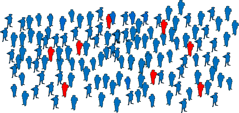
Counts of Diseased People

Counting the people with disease is an important basic measure of disease frequency that is essential to detecting trends or the sudden occurrence of a problem, such as an epidemic. Simple counts of the number of diseased people are also of import to public health planners and policy makers for assessing the need for resources in a population.

Table - New AIDS Cases by Yr

Year	Total AIDS Cases in City A
2001	0
2002	one
2003	5
2004	22
2005	75

The count of AIDS cases shown here for City A would likely stimulate discussion among public officials & health providers, merely count data lone don't allow u.s.a. to fully sympathize the problem. We don't know if all of the cases were long time residents who developed AIDS while living in City A. Some may have moved into town subsequently they developed AIDS. We also don't know whether any of the cases moved away or died.

A second limitation of just counting the number of existing cases is that it doesn't allow us to make fair comparisons of the frequency of HIV in dissimilar cities, since they don't take into account the total number of residents.

When measuring affliction frequency, proportions and rates are very helpful when comparing groups, considering they chronicle the number of people with disease to the size of the population in which they occur.  Prevalence and incidence are the two cardinal measures of disease frequency.

Suppose, for case, that City A had 75 HIV+ residents, while City B had 35. This would suggest a larger problem in City A.

Tabular array - Existing Cases of HIV+ in Cities A and B

	Existing Cases
City A	75
City B	35

All the same, suppose City A was substantially larger, with 30,000 residents, compared to just vii,000 in City B. To exist fair, 1 would need to take this into account by dividing the number of cases in each city by the respective population size.

Table - HIV+ Cases, Population Size, and Prevalence in Cities A and B

	Existing Cases	Population Size	Prevalence
City A	75	30,000	0.0025
Urban center B	35	seven,000	0.0050

In essence, the resulting decimal fractions indicate the frequency of HIV per person in each city, and we can now meet that City B really has a higher prevalence of HIV+ residents than City A, in fact twice equally high (0.005 vs. 0.0025). However, the frequency of HIV per individual is not a very intuitive or useful concept. Nonetheless, if nosotros multiply each of the results x x,000, we have the frequency per 10,000 population. Obviously, neither city has exactly 10,000 residents, but by converting the decimal fractions to this standard population size, nosotros can now have a more understandable description of the prevalence of HIV+ residents in each city.

	Existing Cases	Population Size	Prevalence (as a decimal fraction)	Prevaence (per 10,000 population)
Metropolis A	75	30,000	0.0025	25 per 10,000
City B	35	vii,000	0.0050	50 per 10,000

Prevalence

---

The mensurate of disease frequency nosotros have calculated is the prevalence, that is, the proportion of the population that has disease at a item fourth dimension. Prevalence indicates the probability that a member of the population has a given status at a point in time. It is, therefore, a way of assessing the overall burden of disease in the population, so it is a useful measure for administrators when assessing the need for services or treatment facilities.

Epidemiologists sometimes brand a distinction between point prevalence , the proportion of the population at a 'betoken' in time. So it includes all previous cases who are still have the condition and are still members of the population. A skillful manner to recall nearly point prevalence is to imagine that you took a snapshot of the poplation and adamant the proportion of people who had the condition of involvement at the time the snapshot was taken.

Example: The percentage of a form reporting symptoms of seasonal allergies during the offset week in May 2016.

Period prevalence is similar to betoken prevalence, except that the "point in time" is broader. For instance, suppose that 2,477 residents of Framingham, MA were examined the found the proportion of the population that had cataracts. It may have taken two-3 years to conduct all of the eye exams, and when they were washed the prevalence over this observation flow would include people who had acquired cataracts previously if they still lived in that populations, and it would also include newl cases, i.e., those who had adult cataracts during the 2-3 year flow when the eye exams were conducted. Then, information technology can simply exist thought of equally a wide "point in fourth dimension".

Example: During 1980 the Framingham Het Study examined ii,477 subjects for cataracts and found that 310 had them. So, the prevalence was 310/2,477 = 0.125.

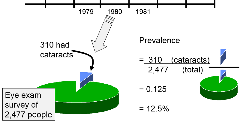
This tin conveniently exist expressed as 12.5 per 100 or 12.5% (per cent means 'per hundred').  Since the examination of these subjects took place over a year, it might be referred to as a period prevalence, and the numerator conceivably could include people who had first developed cataracts prior to 1980 and people who developed cataracts during 1980 just before their exam was washed. Note that all people counted in the numerator are also included in the denominator, i.due east., the numerator is a subset of the denominator.

Often, this stardom betwixt signal prevalence and menstruation prevalence is blurry, because it is rare to exist able to assess the proportion of a population that has a affliction status at exactly the same point in fourth dimension. We could consider our class to be a population, and I could ask the students to raise their mitt if they had an upper respiratory tract infection today. I could fifty-fifty take a photograph and utilize this to visualize the prevalence of respiratory infections at this indicate in fourth dimension. So, in this case this snapshot of disease frequency in the course would truly correspond prevalence at a signal in time. In most cases, withal, it takes much longer than an instant to assess the proportion of a population that is diseased. In other words, we have to exist flexible in our definition of a "point" in time, and nosotros have to let for wide points. Regardless, of this distinction betwixt betoken prevalence and period prevalence, the more than important concept is that prevalence is a measure of the proportion of the population that has a given disease, status, or characteristic at a given time. We will not endeavour to distinguish signal and period prevalence in EP713.

Notes on Prevalence

Note that we can also employ prevalence to appraise the frequency of behaviors or characteristics that might be risk factors for disease. Smoking isn't a disease per se; it is a take chances factor. However, it is relevant to assess the prevalence of this beliefs.

Besides, notation that the "point in time" can be an event rather than a singled-out calendar time. For example, many elderly men are found to have prostate cancer on autopsy, even though they were unaware of information technology and died for other reasons. It is appropriate to think of the frequency of prostate cancer at the time of autopsy as prevalence, even though men are having autopsies performed at many unlike points in agenda time. Similarly, military machine recruits undergo a physical test during induction, and the exams are performed at many different times. Even so, the proportion of inductees constitute to exist colorblind during their physical test would be the prevalence of colorblindness in young men.

 Notation that prevalence is a proportion and not a rate, although the latter term is often used. Then, the terms "prevalence charge per unit" and "autopsy rate" are technically incorrect (although commonly used).

Question: When computing indicate prevalence, what should y'all do with people who were in the population, but they died or moved out of the population?

Answer

Incidence: Hazard, Cumulative Incidence (Incidence Proportion), and Incidence Rate

---

In contrast to prevalence, incidence is a measure of the occurrence of new cases of disease (or some other outcome) during a bridge of time . There are two related measures that are used in this regard: incidence proportion (cumulative incidence) and incidence rate. A useful way to think about cumulative incidence (incidence proportion) is that it is the probability of developing affliction over a stated catamenia of time ; equally such, it is an estimate of risk . Ken Rothman uses the example of a newspaper article that states that women who are 60 years of historic period have a 2% risk of dying from cardiovascular disease. Every bit written this statement is incommunicable to interpret, considering it doesn't specify a fourth dimension catamenia. In order to interpret risk information technology is necessary to know the length of time that applies. A 2% risk has a very dissimilar pregnant if it is over the next 12 months vs. the next 10 years.   Therefore, the incidence proportion (cumulative incidence) must specify a fourth dimension catamenia.   For case, the incidence proportion of neonatal mortality is the number of deaths divided by the number of births over the showtime 30 days after birth.

The concept of risk is fairly intuitive - if a group of disease-free people were followed for a menstruum of time, 1 could determine the proportion of people who developed the illness at some point during the observation period in lodge to make it at an estimate of the probability of developing that illness, i.e. the risk. However appealing this is for its simplicity, there are some drawbacks to this arroyo to assessing the occurrence of health outcomes, because an accurate assessment of probability relies on observing all subjects for the unabridged ascertainment period. This is particularly a problem when assessing long term adventure.

1. First, there are competing risks that might result in the decease of some subjects before the observation period ends, making it impossible to know whether they would accept adult the outcome of involvement if they had non died early on because of some other chance. For example, studying the incidence proportion of long term health conditions amongst soldiers in a conflict zone is complicated by the elevated gamble of dying in gainsay before the effect can exist observed.
2. A second trouble is that, even if subjects don't die for another reason, information technology is difficult to follow people for long periods of fourth dimension, and subjects tin can become lost to follow-upwardly , which also means that their outcome status is unknown.
3. A 3rd trouble is that the incidence proportion doesn't distinguish when a disease occurs equally long as it is inside the follow-up flow.   For example, if a population is followed for 20 years, it would make a difference to the person and to the epidemiologist if the cancer occurred later two years or after xx years, but both of these outcomes would count the aforementioned with the incidence proportion.

For this reason, the incidence proportion is generally used in situations where the follow-upwardly time is relatively short and there is relatively little loss to follow-upward. Otherwise, epidemiologists generally use the incidence rate.

Ideally, if nosotros are to approximate incidence (incidence proportion or incidence charge per unit), we would want to measure this in a sample of people who are truly at run a risk of developing the event of interest. And then, in measuring incidence we would similar to exclude anyone who was not at take chances of developing disease, because they already had the disease or because they couldn't develop it. For case, if one wanted to approximate the risk of developing  uterine cancer in postmenopausal women, we ideally would like to exclude women who had previously undergone hysterectomy (removal of the uterus), since they are no longer at take a chance of developing this item blazon of cancer.

Diabetes in a Nursing Home

Suppose nosotros were interested in the trouble of diabetes in a nursing abode with 800 residents. Nosotros would begin by doing blood tests on all residents to determine which were diabetic. If 50 of the residents were diabetic initially, then the prevalence of diabetes at this betoken in time would be 50/800 = 0.0625. The standard manner of expressing this would exist to say that the prevalence was 62.5 per g residents or vi.25 per 100 residents, or 0.0625%

If nosotros desire to guess the incidence of diabetes in this population over the adjacent 12 months, we demand to exclude the fifty people who are already diabetic and focus on the 750 residents who are disease-free initially. We would then need to do boosted blood tests to determine how many new cases developed during the span of time. Because some of the residents might die or exist transferred to other facilities during the year, we ideally would similar to have claret tests frequently, simply for fiscal and logistical reasons, nosotros might merely behave a second serial of blood tests after one year. If 25 were constitute to be diabetic at the end of a year, then the incidence would be 25/750 = 0.0333 or about 3.three per hundred (3.3%) over a year. Note that we are describing the fourth dimension span, i.e. the flow of observation, when we study the incidence.

When incidence is adamant in this manner, that is, past evaluating the presence of affliction at the commencement and then dividing the number of known new cases by the number of people "at gamble" at the offset, it is referred to as a cumulative incidence and can likewise exist thought of as the incidence proportion . While people ordinarily refer to this every bit a 'rate,' this is really a proportion. It is the proportion of the "at hazard" group that developed disease over a stated block of time.

The cumulative incidence of AIDS in MA during 2004:

Cumulative incidence is like shooting fish in a barrel to measure and is usually used in a wide diverseness of circumstances. For case, if we wanted to determine the incidence of AIDS in Massachusetts during calendar year 2004, it isn't feasible for us to check every citizen at the beginning and finish of the year. Demography data gives us a rough idea of how many people lived in Massachusetts during 2004, and AIDS is a reportable disease, so we could go to the MA Section of Public Health and obtain an estimate of the number of people with AIDS at the beginning of the year, and nosotros could subtract this number from the population size to get a denominator that represents the number of people "at risk" of developing AIDS. Then, nosotros could go back to DPH at the stop of the calendar year and ask how many new people had been reported with AIDS. This is our numerator. So, the cumulative incidence would exist:

(# new AIDS cases reported during the yr) / (population of MA at risk),

i.eastward. minus existing cases at the beginning of the year)

In reality, at that place were 523 new AIDS cases reported in MA in 2004, and the population was well-nigh five.7 meg. So, the cumulative incidence was about 9.ii per 100,000 people during 2004. Note that the denominator is just an estimate based on the last census. In reality, people were being added to and subtracted from the population continually as a effect of births, deaths, moving into the city, and moving out. We too didn't take into account exactly when they developed AIDS, although nosotros probably don't care whether they developed it earlier or later on within a one twelvemonth period. Nevertheless, this cumulative incidence is a useful number, and it is relatively easy to become the information nosotros need to calculate it.

It is important to specify the time period when reporting cumulative incidence. In the fall semester of 2003 there were 130 students in EP713 at the beginning of the semester, and 55 of them reported developing a cold or other respiratory infection during the semester. And then, the cumulative incidence = 55/130 = 0.42307 or 42.3% over the class of the semester. The time period of observation is expressed in words.

Incidence Rate

---

Recall that a charge per unit nearly always contains a dimension of fourth dimension. Therefore, the incidence rate is a mensurate of the number of new cases ("incidence") per unit of time ("rate"). Compare this to the cumulative incidence (incidence proportion), which measures the number of new cases per person in the population over a defined period of fourth dimension. Considering studies of incidence in epidemiology are conducted among groups of people as they movement through fourth dimension, the denominator is actually a combination of the number of people and the amount of time. This is expressed equally person-time. The fourth dimension units can be expressed in days, months, or years, but should exist tied to the length of the study and aid interpretation of the results. The most frequently encountered expression is "person-years". The characteristics of cumulative incidence and incidence rate are illustrated in the examples below.

Annotation: While we more often than not refer to cumulative incidence (incidence proportion) and incidence rate as measures of illness frequency, they tin can be applied to any sort of occurrence. For instance, treatments to cure or relieve disease weather condition are besides measured using the incidence proportion or charge per unit, every bit nosotros will see in the instance below. The cardinal matter to keep in listen is that either measure of incidence (unlike prevalence) measures a transition from 1 state to some other: well to sick, sick to well, alive to dead, unborn to born, etc.

A comparison of pain relief with two analgesics:

Suppose you were asked to clarify the information from a small preliminary clinical trial with twenty subjects. All subjects had a comparable degree of articulatio genus pain from osteoarthritis, and they were existence compared with respect to pain relief after receiving a standard hurting medication (Drug B) or a new pain medication (Drug A). The 20 patients were randomly assigned to one drug or the other, and at that place were ten subjects in each group. Afterwards receiving the medication, the investigators checked on the subjects at hourly intervals to see if the subjects had had relief of hurting. For each field of study, the fourth dimension at which pain relief occurred was recorded. Results are illustrated in the graph below.  Link to a text description of the results

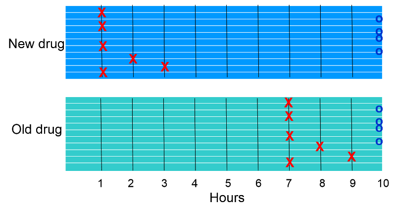
The "X"s indicate when subjects reported pain relief. The "O"s at the finish indicate subjects who did not report relief of pain.

1. Which group appears to have had a greater incidence rate of hurting relief?
2. How did the cumulative incidence of pain relief compare (the proportion of subjects experiencing pain relief)?

Cumulative Incidence

Six of 10 subjects in each group experienced relief of pain, so the cumulative incidence of pain relief was 6/10 = 60% in each group. Whenever cumulative incidence is adamant, ane determines the proportion of subjects who experienced the outcome of involvement during a block of time, without taking into account when subjects adult the outcome. Visually, however, it is articulate that if we consider when subjects experienced relief, the rate was greater in the subjects receiving the new drug.

Incidence Rate

In this hypothetical written report all subjects were observed for a maximum of 10 hours, and some did not accomplish hurting relief, while others got relief after varying periods of time. Nosotros can calculate the average rate of pain relief in each group past adding up the duration of pain for subjects in each group and dividing past the number of subjects in each group.

In the grouping receiving the new drug the times were 4x1 + 2 + 3+ 4x10= 49 hours for the group (person-hours). Then the incidence rate of relief was 6/49 person-hours or on average 12.ii per 100 person-hours of ascertainment. Note that once a subject area experiences the outcome of pain relief, they are no longer considered to exist under observation.

In the group receiving the old drug the times were 4x7 + 8 + ix + 4x10= 85 hours for the group (person-hours). So the incidence rate of relief was six/85 person-hours or on boilerplate 7.0 per 100 person-hours of observation. So, the rate of hurting relief was greater in the group receiving the new drug.

What we have calculated is the incidence charge per unit . This is a truthful rate, considering time is an integral part of the calculation, coordinating to miles per hour (a rate of speed) or gallons per minute (a rate of flow).

Several things are noteworthy nigh this incidence rate.

1. The numerator is the aforementioned for both cumulative incidence and incidence charge per unit; information technology is the number of individuals who adult the outcome of interest (in this case pain relief) during the observation period.
2. The denominators for cumulative incidence and incidence rate are very different. For cumulative incidence, the denominator is the total number of "at risk" subjects being followed; for incidence rate, the denominator is the total corporeality of time "at risk" of connected pain for all the subjects who were being followed. Therefore, nosotros tin only summate an incidence rate if nosotros have periodic follow-upwards information on each subject, including not only if they adult the result, merely also when they adult it.
3. The incidence rate is a more accurate estimate of the rate at which the result develops. Cumulative incidence is ofttimes referred to as a 'rate', but it actually is the proportion of people who develop the upshot during a stock-still cake of time. This was useful when we wanted to draw the incidence of AIDS in Massachusetts, considering we didn't have detailed information on each and every resident of the land. We couldn't take into account when people developed AIDS. Moreover, nosotros couldn't account for people who moved into the state in the middle of the year or people who moved out or died. With incidence rate, however, nosotros can accept these factors into account. The strategy is the aforementioned as in the hurting relief sample above, i.e. the denominator takes into account the total amount of "at risk" time for the grouping.
4. Incidence rates are especially advantageous when trying measure incidence in studies with dynamic populations and in studies with fixed populations with relatively long follow-upwardly fourth dimension.

Question: A participant in a prospective cohort study or a randomized clinical trial stops contributing additional "disease-free observation time" when they develop the outcome of involvement or go lost to follow-upwards for whatever reason (death, failure to respond to telephone calls, letters and emails, etc.). Does this hateful that they are no longer in the study?

Answer

Incidence of HIV in a Brothel

A follow-up study was conducted to determine which sexual behaviors were associated with the greatest risk of becoming HIV+. The study was conducted in a group of female prostitutes. The subjects were tested prior to the kickoff of the study, and 5 HIV+ women were excluded. The the remaining x women were followed for six years beginning in Jan 1989. Each woman was contacted and retested at the beginning of Jan each year. The table beneath summarizes the findings these ten subjects. A circled plus sign (+) indicates when a subject area was found to be HIV+; a question marker (?) indicates when a subject became lost to follow-upwardly. The dashed lines indicate continued follow-up.

Link to a detailed description of the table below

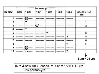
The cumulative incidence was iv/10=40% over six years, just this doesn't take into business relationship the different amounts of time contributed by those who didn't become HIV positive, one of whom (Subject #vii) was followed throughout the six years of the study, but the remainder of whom were lost to follow-up sometime before the end of the study (Subjects #ii, four, five, 6, 8).

The incidence charge per unit , still, can take these problems into account, because the denominator is the total "at risk" observation time contributed by all ten subjects. The column at the far right indicates each subject's "at take chances" observation time, and the sum for the ten subjects was 26 years. So, the IR= 4/26 person-yrs = 0.xv/person-twelvemonth = 15/100 person-years of observation.

Annotation that person-time stopped beingness counted every bit soon as the field of study was establish to exist HIV positive, because the subject was no longer "at hazard" of developing the outcome—they already had experienced it.   For case, Subject field #1 contributed one person-yr even though she was followed for all half-dozen years.

Incidence rates are often computed in prospective cohort studies (e.g., The Framingham Heart Study or The Nurses Health Report) and randomized clinical trials (east.g., The Md's Health Report, which looked at the effect of depression-dose aspirin on centre affliction). It is more accurate than cumulative incidence, simply it requires repeated follow-up observations on each discipline, and studies similar this can be very expensive and time consuming.

Also consider that subjects are sometimes recruited into studies at unlike times. Each subject field's disease-free observation time or "at adventure" fourth dimension can be calculated as the fourth dimension from their entry into the written report until a) they get the affliction, b) they become lost to follow-up, or c) the study ends.

For example, consider a hypothetical clinical trial that was conducted to decide whether taking low-dose aspirin reduced the frequency of centre attacks in center-anile and elderly men. The time line below summarizes events 12 subjects labeled one-12, all of whom were allocated to the placebo-treated grouping.

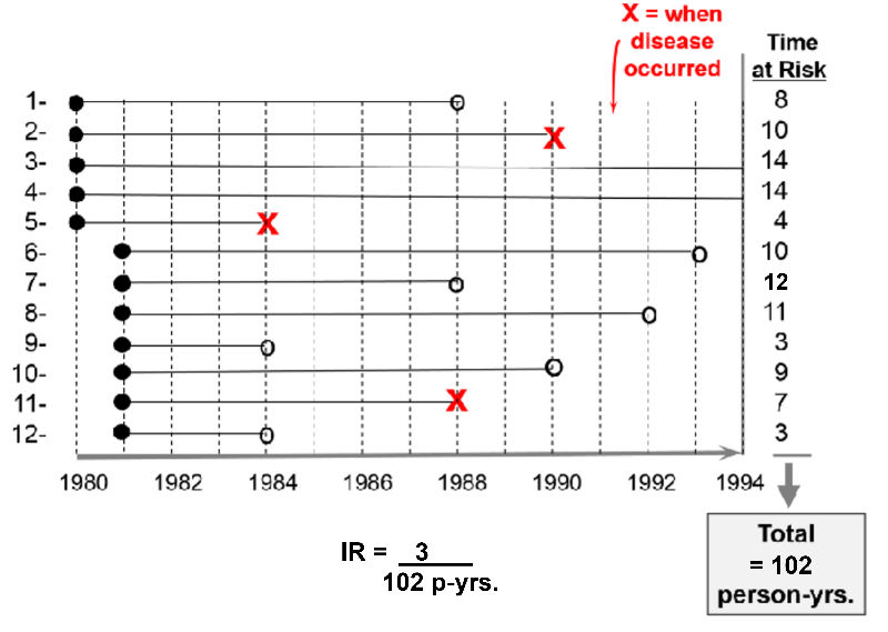
The kickoff five subjects were enrolled in 1980, and the next 7 subjects were enrolled 1 year later. All subjects began taking aspirin upon enrollment. Therefore their "exposure" to aspirin began upon enrollment as indicated by the solid black dots.

The carmine "X"due south bespeak when subjects had a heart attack; their exposure time at take a chance ends there, since having a outset heart assail means that they were no longer at risk of having a first center attack; they had the result of interest at that betoken. Subject area #two had a heart set on in 1990; subject #v had one in 1984; bailiwick #11 had one in 1988.

The open circles indicated six subjects who were lost to follow-upward. They stopped responding to all requests for follow up later on that indicate. We know that they had not had a heart attack up to that bespeak, only we don't know what happened to them later that, so they terminate contributed observed exposure time at risk. Subject #one was lost to follow up in 1988; #half-dozen was lost in 1993; #7 was lost in 1988; #8 was lost in 1992; #nine was lost in 1984;

All of this information can be taken into business relationship in guild to compute the average rate at which middle attacks occur in this group of 12 men beingness treated with low-dose aspirin. We tin practice this in a way that is analogous to example #2 in a higher place. There were 3 heart attacks, and nosotros divide this past the total corporeality of time that the men were exposed and at run a risk of developing a heart assault. For each homo the exposure time at risk is the time from their entry into the study until one of iii endpoints: a) the disease occurs, b) the subject is lost to follow-upward, or c) the study concludes. The exposure fourth dimension at risk for each man is shown in the column at the far right of the effigy, and if we add these, the total exposure time for the group was 102 years. Therefore, the average charge per unit at which the outcome occurred was iii/ 102 person-years of observed exposure time.

Example: Incidence Rate in the Nurse'southward Health Written report - Estrogens and Coronary Artery Illness

Data collected from the Nurses' Wellness Report, a prospective cohort study, was used to compare rates of coronary avenue illness in post-menopausal women using hormone replacement therapy (HRT) and post-menopausal women who had not used HRT. The data was summarized in the table beneath.

	Coronary Avenue Disease	Person-Years of Disease Free Ascertainment
Used HRT	30	54,308.vii
No Use of HRT	60	51,477.5

Women on postmenopausal hormones had an incidence rate of 30 events during 54,308.seven person years of follow-up, or 55.2 / 100,000 person-years. Women in the untreated group had sixty events during 51,477.5 person-years of follow-upward - an incidence rate of 116.half dozen / 100,000 person-years.

Another Example: Incidence Rate in the Nurse's Health Study – Obesity and Myocardial Infarction

In this study, incidence rates of MI (myocardial infarction) were compared among five groups of women based on their body mass index (BMI). In that location were certainly dissimilar numbers of women in the 5 groups, but for each group they computed the incidence charge per unit past counting the number who adult MI and dividing by the group's total "at risk" time of observation. The event was and then converted to the number per 100,000 person-years to facilitate comparison among the five groups.

Body Mass Index (BMI)	# Non-fatal Myocardial Infarctions	Person-Years of Observation	Incidence Charge per unit per 100,000 Person-Years
<21	41	177,356	23.1
21.0-22.9	57	194,243	29.3
23.0-24.9	58	155,717	36.0
25.0-29.nine	67	148,541	45.i
> 30	85	99,573	85.4

Units for Denominators

By convention, all iii measures of disease frequency (prevalence, cumulative incidence, and incidence rate) are expressed as some multiple of x in gild to facilitate comparisons. Consider these 3 examples:

• Cumulative incidence: iv/10 over vi years = 0.40 = 40 per 100 or twoscore% over vi years
• Incidence rate: 3/107.7 person-yrs = 0.02785/person-year = 28 per 1,000 person-years

One can express the concluding result equally the number of cases per 100 people, or per one,000 people, or per x,000 people, or per 100,000. Generally ane uses a convenient multiple of ten. For example, the expressions below are all equivalent, but the last two are the most user-friendly to talk about & think about. Note: Each time you movement the decimal to the right, you increase the number by a factor of ten.

Equivalent Expressions of Disease Frequency

0.00232 new cases per 1 person-yrs.

    0.0232 new cases per 10 person-yrs.

    0.232 new cases per 100 person-yrs.

    2.32 new cases per 1,000 person-yrs.

  23.2 new cases per 10,000 person-yrs.

232 new cases per 100,000 person-yrs.

Common Pitfall : A common mistake amid offset students is to fail to specify the dimensions after calculating incidence, especially for cumulative incidence.

• In the example for HIV in sex activity workers, the incidence charge per unit should be reported as xv per 100 person-years. Notation that this number is non the equivalent of a percentage.

• In the aforementioned example, the cumulative incidence was iv per 10 subjects (40%) over 6 years. Note: You must specify the fourth dimension period for cumulative incidence or you lot volition lose points on the exams.

Summary of Basic Measures of Disease Frequency

Prevalence (a proportion)

    = People # People with affliction at a point in fourth dimension

       Full People  # People in the study population

Cumulative Incidence (a proportion)

    = People # new cases in a specified period

        Total People  # People (at gamble) in the study population

Incidence Rate (a charge per unit)

     = People # new cases of illness

   People-Time         Total observation time in a group at hazard

Human relationship of Incidence Rate to Cumulative Incidence (Risk)

---

Cumulative incidence (the proportion of a population at risk that volition develop an consequence in a given menstruum of time) provides a measure of risk, and it is an intuitive way to think about possible health outcomes. An incidence rate is less intuitive, because it is really an approximate of the instantaneous rate of disease, i.e. the rate at which new cases are occurring at whatsoever item moment. Incidence charge per unit is therefore more than analogous to the speed of a auto, which is typically expressed in miles per hr. Time has to elapse to measure a car's speed, but nosotros don't have to wait a whole hr; nosotros can glance at the speedometer to come across the instantaneous charge per unit of travel. Rather than measuring risk per se, incidence rate measures the rate at which new cases of disease occur per unit of time, and time is an integral part of the calculation of incidence rate. In dissimilarity, cumulative incidence or take a chance assesses the probability of an issue occurring during a stated menstruum of observation. Consequently, it is essential to depict the relevant time menstruum in words when discussing cumulative incidence (gamble), merely time is non an integral role of the calculation. Despite this distinction, these two ways of expressing incidence are apparently related, and incidence rate can be used to estimate cumulative incidence. At first glance it would seem logical that, if the incidence rate remained constant the cumulative incidence would be equal to the incidence rate times time:

CI = IR x T

This relationship would hold true if the population were infinitely large, only in a finite population this approximation becomes increasingly inaccurate over time, because the size of the population at risk declines over time. Rothman uses the example of a population of i,000 people who feel a bloodshed rate of xi deaths per ane,000 person-years over a menses of years; in other words, the rate remains abiding. The equation above would lead the states to believe that after 50 years the cumulative incidence of decease would be CI = IR X T = xi X 50 = 550 deaths in a population which initially had one,000 members. In reality, there would only exist 423 deaths after 50 years. The problem is that the equation above fails to take into business relationship the fact that the size of the population at risk declines over time. After the commencement year in that location have been xi deaths, and the population now has only 989 people, not 1,000. As a result, the equation higher up overestimates the cumulative incidence, because there is an exponential disuse in the population at risk. A more than accurate mathematical expression that takes this into account is:

CI = 1 - e^{(-IR x T)}, where 'e' = ii.71828

This abiding 'e' arises in many mathematical relationships describing growth or decay over time. If you are using an Excel spreadsheet, you could calculate the CI using the formula:

CI = one - EXP(-IR xT)

In the graph below the upper blueish line shows the predicted number of deaths using the approximation CI = IR x T. The lower line, in ruby-red, shows the more accurate projection of cumulative deaths using the exponential equation.

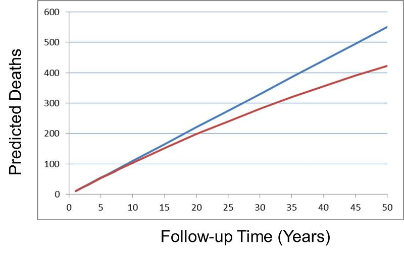
Withal, note that the prediction from CI = IR x T gives quite reasonable estimates as long as the cumulative incidence remains less than ten% (equivalent to 100 deaths in the population of 1,000 in the to a higher place graph).

Life Tables and Survival Analysis

---

(Optional)

The equation CI = IR x T provides a reasonable judge of run a risk when the incidence rate is relatively abiding, but this isn't always the case. When the incidence rate changes over fourth dimension there are other options for estimating risk.

1. 1 could calculate gamble serially over shorter time intervals during which risk is reasonably abiding. However, the intervals have to be long enough to enable meaningful incidence rates for each interval.
2. Another arroyo that is useful when risk is changing over fourth dimension is to employ survival analysis . Despite the proper noun, it can exist used for any upshot regardless of whether it is fatal or non. The table below shows a hypothetical life-table cited by Rothman.

Table - Life-table for Death from Motor-vehicle Injury from Bitth through Age 85

Historic period (years)	Mortality Charge per unit per 100,000 person-years	At Run a risk	Deaths in Interval	Take a chance	Survival Probability	Cumulative Survival Probability
0-14	4.7	100,000	70.v	0.000705	0.999295	0.999295
xv-24	35.nine	99,930	358.1	0.003584	0.996416	0.995714
25-44	20.1	99,571	399.5	0.004012	0.995988	0.991719
45-64	18.4	99,172	364.three	0.003673	0.996327	0.988077
65-84	21.seven	98,808	427.9	0.004331	0.995669	0.983798

Adapted from Iskrant and Joliet

In this hypothetical example, the initial population at chance was arbitrarily gear up at 100,000, and the mortality rates in each group (column 2, mortality rates=deaths per 100,000 person-yrs.) were used to calculate the number of deaths among those remaining at risk for each interval using the formula CI = IR x T. Thus, the first historic period group spanned 15 years and the mortality charge per unit was four.7/100,000 person-years, then the number of deaths was 4.7 x xv = seventy.v.

The illustration beneath shows the results of analysis of a trial looking at the ability of zidovudine (an anti-retroviral drug used in the treatment and prevention of HIV) to reduce maternal to child transmission. Pegnant women with mildly symptomatic HIV disease and no prior treatment with antiretroviral drugs during the pregnancy, were randomly assigned to one of ii regimens: i) a regimen consisting of zidovudine given ante partum and intra partum to the mother and to the newborn for six weeks or 2) placebo.

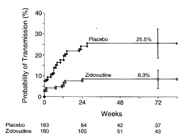
The graph shows that about eight % of the infants in the placebo group tested HIV+ at nascence, and the probability of HIV transmission in this group rose to 25.5% by 72 weeks of age. Infants in the zidovudine grouping just had well-nigh a 3% probablility of being born HIV+, and their risk of transmission only todr yo 8.3% by 72 weeks of age. (The data are from Connor EM, et al.: Reduction in maternal-infant manual of man immunodeficiency virus type one with zidovudine treatment. North. Engl. J. Med. 1994;331:1173-1180, as quoted in the textbook past Aschengrau and Seage in Table 7-5, page 191 in the 2d edition.) This was part of protocol 076 that originally demonstrated the efficacy of zidovudine in women in the United States and French republic. The illustration below shows Kaplan-Meier plots of the probability of HIV transmission for the ii groups. The estimated percentages of infants infected at 72 weeks are shown with 95 percent confidence intervals. The numbers of infants at risk at 24, 48, and 72 weeks are shown below the figure.

Human relationship Among Prevalence, Incidence Rate, and Average Elapsing of Disease

---

Prevalence is the proportion of a population that has a condition at a specific fourth dimension, only the prevalence will be influenced past both the rate at which new cases are occurring and the average duration of the disease. Incidence reflects the rate at which new cases of disease are being added to the population (and becoming prevalent cases). Average duration of disease is besides of import, considering the only mode you can stop beingness a prevalent instance is to be cured or to move out of the population or die. For example, about a decade ago the average duration of lung cancer was almost six months. Therapy was ineffective and about all lung cancer cases died. From the time of diagnosis, the average survival was but nigh six months. And so, the prevalence of lung cancer was fairly low. In contrast, diabetes has a long average duration, since information technology tin can't exist cured, but it tin be controlled with medications, and then the average elapsing of diabetes is long, and the prevalence is adequately high.

If the population is initially in a "steady country," pregnant that prevalence is fairly abiding and incidence and outflow [cure and decease] are nearly equal), and so the relationship among these three parameters can be described mathematically every bit:

P/(1-P) = IR 10 Avg. Duration ,

where P= proportion of the population with the disease and (one-P) is the proportion without information technology, IR is the incidence rate, and Avg. Duration is the average time that people take the affliction (from diagnosis until they are either cured or die). If the frequency of affliction is rare (i.e., <10% of the population has it), and then the relationship can be expressed as follow:

Prevalence = (Incidence Rate) x (Average Duration of Affliction)

• If the average duration of disease remains abiding, then preventive measures that reduce the incidence of affliction would be expected to result in a decreased prevalence.
• Similarly, if the incidence remained constant, then developing a cure would reduce the average duration of illness, and this would also reduce the prevalence of disease.
• In the late 1990s anti-retroviral therapy was introduced and profoundly improved the survival of people with HIV. However, they weren't cured of their disease, meaning that the average duration of disease increased. Every bit a consequence, the prevalence of HIV increased during this catamenia.

The relationship tin can be visualized by thinking of inflow and outflow from a reservoir. The fullness of the reservoir can exist thought of as analogous to prevalence. Raindrops might represent incidence or the rate at which new cases of a illness are being added to the population, thus becoming prevalent cases. Water also flows out of the reservoir, analogous to removal of prevalent cases past virtue of either dying or existence cured of the illness. Imagine that incidence (rainfall) and the rate of cure or decease are initially equal; if so, the top of h2o in the reservoir will remain constant.

• If outflow from the reservoir (rates of cure or death amid prevalent cases) remains constant and rainfall (incidence of new disease) increases, then the height of water in the reservoir volition ascension. Conversely, if incidence (rainfall) declines, and so the water level will autumn.
• If we start from steady state again, and the rate of rainfall remains constant, but the outflow (charge per unit of cure or charge per unit of death) increases, so the height of the water (prevalence) will fall. Conversely, if incidence is held abiding, but outflow falls (due east.k., if the lives of prevalent cases are prolonged, but they aren't cured, then the height of the water will rise.

Calculating Average Duration of Affliction

This relationship can as well be used to calculate the average elapsing of illness under steady state circumstances. If Prevalence = (Incidence) 10 (Boilerplate Duration), and then it follows that

Average Elapsing =  (Prevalence) / (Incidence)

Example: Suppose the incidence rate of lung cancer is 46 new cancers per 100,000 P-Y, and the prevalence is 23 per 100,000 population, then

Average Duration of Disease = (23/100,000 persons /  46/100,000 person-years  = 0.5 year

Conclusion: Individuals with lung cancer survived an average of 6 months from the fourth dimension of diagnosis to death.

Special Types of Frequency Measures

---

Prevalence and incidence are the fundamental measures of disease frequency, but special names have evolved for these measures, depending on their specific utilize. All of these tend to exist referred to as rates, even though, strictly speaking, they often refer to proportions (cumulative incidence or prevalence).

Category-specific Rates

Either prevalence or incidence can be broken down into categoies, e.g., historic period groups, or past gender, or race, or some combination of these. For instance, since disease frequency often differs substantially with historic period, 1 frequently sees "age-specific" rates of disease.

Example 1: A tabular array of age-specific rates of stroke (incidence)

Age Group	# New Occurrences	Group Size	Cumulative Incidence per 100,000 persons
0-34	0	582,083	0
35-44	28	113,581	25
45-54	114	114,208	100
55-64	320	91,484	350
65-74	550	81,155	900
75+	one.126	37,531	iii,000

Case 2: A Table of race-specific causes of expiry per 100,000 population (mortality rates, i.e., incidence) in the United states, 1967

	White	Black
Hypertension	21.i	68.6
Homicide	3.v	32.3
Diabetes mellitus	16.6	28.9
Tuberculosis	2.5	9.six
Suicide	11.iii	v.7
Leukemia	7.four	5.5
Syphilis	1.0	3.0

Interesting Visual Tour of Causes of Death in the US

Special Measures of Incidence

Morbidity rate is the incidence of non-fatal cases of a disease in a population during a specified fourth dimension menstruation. For case, during 1982 in that location were 25,520 non-fatal cases of TB in the US population. The mid-yr population was estimated at 231,534,000. Therefore, the

Morbidity rate of TB =25,520/231,534,000  = 11.0/100,000 over ane year

Note that this is a cumulative incidence and therefore is really a proportion, not a true rate.)

Mortality Rate: In 1982 in that location were i,807 deaths from TB in the US population, and so the bloodshed rate for TB was vii.8 per meg over one year (also a cumulative incidence, not a true rate).

Instance-Fatality Rate: the number of deaths from a specific disease divided by the total number of cases of that disease, i.e. the proportion of fatal cases of a disease (%). This provides a measure of the severity of the illness.

Instance: Reyes Syndrome is a rare, but highly fatal disease in which the liver and brain get dysfunctional due to aberrant accumulation of cellular fat. It tends to occur when people are recovering from a viral illness, and information technology tends to exist associated with use of aspirin, especially in children. If in that location were 200 cases of Reyes syndrome in 1982 and 70 died, then the instance-fatality rate would be 70/200 = 35% over one yr.

[Note: This is generally calculated by dividing the deaths reported in a given yr by the number of cases reported in the same year, just this can be misleading since some diseases (due east.thou., TB) aren't quickly fatal. Thus, many of the TB fatalities that occurred in 1982 were due to cases diagnosed several years before.]

Attack Rate: a cumulative incidence for a disease during a specific menstruum (e.g., an epidemic).

Example: Later a church picnic in Oswego, NY many attendees got food poisoning. In that location were 75 people at the picnic; 46 got ill inside several hours, then the attack charge per unit was 46/75 = 61%.

Live nascence rate: the frequency of alive births in one yr per ane,000 females of childbearing age.

Infant Mortality Rate: the frequency of deaths in children nether 1 twelvemonth of age occurring during a one year period per 1,000 live births.

Special Prevalence Measures

These are often incorrectly referred to as incidences or rates, merely they are, in fact, proportions..

Autopsy Rate : the proportion of people who have a particular finding on a postmortem exam (the prevalence of a certain finding among the population of people who get autopsied).

Nativity Defect Charge per unit : the prevalence of a built aberration at the "betoken" of nativity. The denominator can be either live births or full births (which includes live births + stillbirths), but it generally does not include spontaneously aborted fetuses.

The Obstacle Course

---

Questions to examination your agreement

A sample of 100 middle aged and elderly women was followed prospectively for 10 years in order to study rates of ovarian cancer. All subjects entered the study on January 1, 1990, and all were free of cancer at the kickoff. All women were followed until December 31, 1999. None were lost to follow-up. During this period, five subjects were diagnosed with ovarian cancer, but they all survived to the terminate of the study.

Instance #1 was diagnosed with ovarian cancer in January 1991.

Case #2 was diagnosed in Jan 1992.

Case #3 was diagnosed in January 1993.

Instance #4 was diagnosed in Jan 1986.

Instance #five was diagnosed in January 1996.

The time at which these 5 subjects developed cancer is shown in this table:

Use this data and the information in the table below to respond the questions beneath the tabl:

Subject	1990	1991	1992	1993	1994	1995	1996	1997	1998	1999
Example #one		cancer
Example #2			cancer
Case #iii				cancer
Case #4							cancer
Case #5									cancer

Utilize this information and the data in the table below to reply the questions below the table:

In January of 1990, one,010 young adults offered to participate in a ten-year prospective report to make up one's mind their adventure of Blazon-I diabetes.  This group underwent an initial blood test to determine whether they were diabetic, and eligible subjects were re-tested yearly for the side by side 10 years. Amidst the group that offered to join the report:

• At that place were 2 individuals who were found to have diabetes on the initial blood screening; these 2 people were referred for treatment and were not enrolled in the study
• There were i,000 who were illness-free and remained disease-complimentary for the entire 10 years of the study
•  6 individuals adult diabetes during the grade of the study at the times indicated in the table below
•  2 individuals who were initially disease-free were lost to follow-up during the study at the times indicated in the table beneath

 ?  = Lost to follow-up        + = Claret examination positive for diabetes         ------ = Continued disease-free follow-up

Bailiwick #	1990	1991	1992	1993	1994	1995	1996	1997	1998	1999
1	------	------	+
2	------	------	------	------	------	------	------	------	------	+
3	------	------	------	------	------	------	------	+
4	------	+
5	------	------	------	------	+
6	------	------	+
7	------	------	------	------	?
8	------	------	------	------	------	?

Source: https://sphweb.bumc.bu.edu/otlt/mph-modules/ep/ep713_diseasefrequency/ep713_diseasefrequency_print.html

Posted by: hernandezdencen.blogspot.com

Share this post